organic solar cells – Notes on Disordered Matter

Looking for Postdoc for Simulation/ML and Experimentation – Printed Organic Solar Cells

Rod MacKenzie and I are looking for a postdoctoral researcher, POPULAR yellow sun. mainly for doing device simulations with Rod’s OghmaNano combined with machine learning. The position is for more than 2 years, at TU Chemnitz in Germany. We have a strong collaborative team beyond our groups, within the DFG Research Unit P☀PULAR on printed organic solar cells and the ChemDeTOX project on chemical defects in conjugated polymers. If you are interested, please find the details on the TU Chemnitz job portal (German and English).

How to see the temperature dependence of the open-circuit voltage from the ideal diode equation?

The open-circuit voltage is the voltage in the current–voltage characteristics of a solar cell that is defined where the current is zero. That means that the (internal) charge carrier generation and recombination rates are equal, so that no net current can flow out of the device.

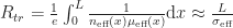
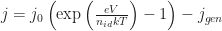
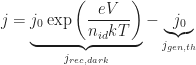
We can simply rearrange the ideal diode equation and solve for the open-circuit voltage. The ideal diode equation was discussed with respect to the ideality factor in this post. The current density is given as

$j(V)=j_0 \left(\exp\left(\frac{eV}{n_{id}kT}\right)-1\right) - j_\text{gen}$ ,

with $V$ the voltage, $e$ elementary charge, $kT$ thermal voltage, $n_\mathrm{id}$ the recombination ideality factor, $j_0$ the dark saturation current, and $j_\mathrm{gen}$ the photogenerated current. For simplicity, the latter is chosen to be voltage independent, and therefore is equal to the short-circuit current $j_\mathrm{sc}$ .

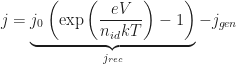
As the open-circuit voltage is determined at zero net current, $j(V_\mathrm{oc}) = 0$ , we get

$j(V_\mathrm{oc}) = 0 = j_0 \left(\exp\left(\frac{eV_\mathrm{oc}}{n_{id}kT}\right)-1\right) - j_\text{gen}$ ,

which we can rearrange to yield the open-circuit voltage

$V_\mathrm{oc} = \frac{n_{id}kT}{e} \ln \left( \frac{j_\text{gen} + j_0}{j_0} \right)$ .

Here, $j_\text{gen}$ is the photocurrent due to solar illumination, and the dark saturation current density $j_0$ is due to excitation of thermal “black body” photons from the ambient at, say, room temperature. In the simplest case – in the dark where $j_\text{gen} = 0$ – we see that $V_\mathrm{oc} = 0$ , too. Generally, the thermal generation leading to $j_0$ is much weaker than the solar generation $j_\text{gen}$ , therefore

$V_\mathrm{oc} \approx \frac{n_{id}kT}{e} \ln \left( \frac{j_\text{gen}}{j_0} \right)$ .

is usually a very good approximation.

This simple equation to describe the open-circuit voltage is very general and can describe (outside of the shunt region, which is not considered here) very different solar cell technologies correctly. The reason is that many parameters that differ for different semiconductors are accounted for. So what determines the open-circuit voltage?

At a given temperature, the open circuit voltage is determined by
– $j_\text{gen}$ ,
– $j_0$ , and
– $n_\text{id}$ (which was discussed previously)..

The generation current density

$j_\text{gen} = e \int EQE(E)\, b_s(E)\, dE,$

which means it is given by how much of the solar photon flux of the sun, $b_s$ , is converted into electrons – which is described by the external quantum efficiency $EQE(E)$ . The $EQE$ includes reflection losses, the absorptance (in the simplest case 0 below the bandgap and 1 for energies at or higher than the band gap $E_g$ ), and charge collection losses (for instance due to the transport resistance). Essentially, the higher the bandgap $E_g$ , the higher $j_\text{gen}$ – which leads to a higher open-circuit voltage.

The dark saturation current density in an ideal solar cell without non-radiative losses is essentially given by

$j_0 = e \int EQE(E)\, b_a(E)\, dE.$

The only difference to the equation for $j_\text{gen}$ is that the photons do not come from the sun anymore, but from the ambient (note the subscript a;). This $b_a(E)$ is just Planck’s law to describe thermal radiation from black bodies, so everything “earthly” around the solar cell that emits at the current temperature $T$ (or $T_a$ , the temperature of the ambient). While the sun that generates $j_\text{gen}$ can also be well approximated by a block body and Planck’s law – assuming a black body temperature of the sun of $T_s \approx 5800 \text{ K}$ , usually the temperature of the ambient that leads to $j_0$ corresponds to the solar cell temperature… for instance, $T = T_a \approx 300 \text{ K}$ .

With this in mind, we can maybe see already what determines the temperature dependence of the open-circuit voltage! In

$V_\mathrm{oc}(T) \approx \frac{n_{id}(T)kT}{e} \ln \left( \frac{j_\text{gen}}{j_0(T)} \right)$ ,

there is an explicit temperature dependence in the prefactor, $kT$ , which “promises” increasing open-circuit voltages at higher temperatures, but from measurements we know that the opposite happens: the open-circuit voltage increases towards lower temperatures!

Except for temperature-dependent changes in the charge collection (or bandgap), $j_\text{gen}$ is (solar cell) temperature independent. The ideality factor can depend on temperature (and, in organic solar cells, even light intensity dependence [Saladina 2023]), but does not dominate the temperature dependence of $V_\mathrm{oc}$ . The real “culprit” is indeed the very important dark saturation current density $j_0$ , which describes charge carrier generation (and recombination!) across the bandgap by thermal photons (plus, in real systems, non-radiative processes)!

When we approximate the equation for the ideal dark saturation current density (ideal, because we again neglect non-radiative losses) from above – using the Boltzmann approximation instead of the Bose-Einstein statistics that are featured in Planck’s law – we can describe the temperature dependence of $j_0$ :

$j_0(T) \approx j_{00} \exp \left( - \frac{E_g}{n(T)kT} \right) \qquad \mathrm{(*)}$ .

The temperature here is, again, the solar cell’s and the ambient temperature is equal to it. We assume for simplicity (again a pretty good approximation) that the bandgap $E_g$ is not (or only very weakly) temperature dependent. The prefactor $j_{00}$ is essentially the dark saturation current density at infinite temperature, when the effective density of states is (hypothetically) completely filled, which is reduced by lower temperatures: the thermal photons from the ambient generate electron–hole pairs across the bandgap, increasing $j_0$ and – as it is in the denominator of the equation for $V_\mathrm{oc}$ – decreasing the open-circuit voltage at higher temperatures. We can make this result more transparent when entering the temperature dependent dark saturation current density into the equation for the open-circuit voltage: (For simplicitly, I left the explicit temperature dependence of the ideality factor out, writing $n_{id}$ instead of $n_{id}(T)$ .)

$V_\mathrm{oc}(T) \approx \frac{n_{id}kT}{e} \ln \left( \frac{j_\text{gen}}{j_{00} \exp \left( - \frac{E_g}{n_{id}kT} \right)} \right)$
$= \frac{n_{id}kT}{e} \ln \left( \frac{j_\text{gen}}{j_{00}} \exp \left(\frac{E_g}{n_{id}kT} \right) \right)$
$= \frac{n_{id}kT}{e} \ln \left( \exp \left(\frac{E_g}{n_{id}kT} \right) \right) + \frac{n_{id}kT}{e} \ln \left( \frac{j_\text{gen}}{j_{00}} \right)$
$= \frac{n_{id}kT}{e} \frac{E_g}{n_{id}kT} + \frac{n_{id}kT}{e} \ln \left( \frac{j_\text{gen}}{j_{00}} \right)$
$= \frac{E_g}{e} + \frac{n_{id}kT}{e} \ln \left( \frac{j_\text{gen}}{j_{00}} \right)$

We see now that the maximum open circuit voltage at zero temperature (in a system described by classical Boltzmann approximation, Voc(T) for a-Si H solar cell. i.e. without the energetic disorder that is an important topic in organic solar cells) is given by the (effective) bandgap of the device – usually the bandgap of the active layer material. The open-circuit voltage is reduced at higher temperatures(!) despite the plus sign after the term $E_g/e$ : the dark saturation current density at infinite temperature $j_{00}$ is larger than $j_\mathrm{gen}$ , and the argument of a natural logarithm with argument smaller than one is negative. This means that the second term on the right-hand side is negative, and $V_\mathrm{oc}$ decreases at higher temperatures.

I’ll leave it here for now, with two comments: first, there is more to be said about why one always should use the ideality factor in the equation $\mathrm{(*)}$ that gives the temperature dependence of the dark saturation current density! And second, the impact of energetic disorder on $V_\mathrm{oc}$ is very important and leads to changes – the devil in the details;)

The transport resistance in organic solar cells

In one of my last posts on the diode ideality factor (6 years ago…), I promised to talk about the transport resistance in organic solar cells. I came across it already during my time at IMEC in Leuven, Belgium, around 2004: my colleagues and I worked on an analytic model of the open circuit voltage in organic bilayer solar cells. The corresponding paper was published a few years later, [Cheyns et al 2008], but I have to admit that I did not grasp its importance as a relevant loss mechanism for organic solar cells in general, focussing on geminate and nongeminate recombination – until this paper by [Würfel/Neher et al 2015] came out. I think now I have;)

The transport resistance is an internal resistance in the active layer (or transport layer(s)) of the solar cell, acting like an internal series resistance: It changes the slope of the current density–voltage characteristics – for instance around the open circuit voltage – and thus reduces the fill factor.

If you can live with an effective conductivity $\sigma_\text{eff} = e n_\text{eff} \mu_\text{eff}$ for now, I’d say that the transport resistance is given as

$R_{tr}= \frac{1}{e} \int_0^L \frac{1}{n_\text{eff}(x) \mu_\text{eff}(x)} \text{d}x \approx \frac{L}{\sigma_\text{eff}}$

with the effective carrier concentration $n_\text{eff}$ , the effective mobility $\mu_\text{eff}$ , and the active layer thickness $L$ . For a finite current $j$ , the externally applied voltage $V_\text{ext}$ of the $j(V_\text{ext})$ curve (red in the sketch) losses in current-voltage characteristics is reduced by $\Delta V = V_\text{ext} - V_\text{int} =j R_{tr}$ as compared to the transport resistance free case which I call $j(V_\text{int})$ (violet). The reason is that the electron and hole energy levels equivalent to conduction and valence band are more tilted due to the influence of the low conductivity. Rod MacKenzie from Durham used his drift–diffusion simulation programme gpvdm – which among many other features allows to use the multiple-trapping-and-release model to account for energetic disorder – to calculate an example. In the figure, the energy levels corresponding to conduction and valence band are shown, and the yellow shading between the band edges correspond to the trap populations which I will ignore. So focus on the edges! Band bending due to transport resistance, by Rod MacKenzie using gpvdm The upper left inset features the band bending of the transport resistance free case at a current–voltage point in the fourth quadrant of an illuminated solar cell, $V_\text{int}$ being at 0.8 V. The red lines show that in the bulk, the bands are perfectly flat despite not being at any “flat band” voltage. In contrast, the lower left inset shows the band bending for the illuminated current–voltage point at the same current, but at $V_\text{ext}$ of 0.69 V. The voltage difference $\Delta V$ of 0.11 V is due to the transport resistance. The two perfectly horizontal red lines, just shifted down from above, now show a discrepancy due to the band bending in the bulk. This tilt sums up to the voltage loss $\Delta V$ , and corresponds to a gradient of the quasi-Fermi levels, as discussed clearly in [Würfel/Neher et al 2015] around Eqn (8). Let me note that the denomination of $V_\text{int}$ as opposed to $V_\text{ext}$ is a bit unfair, as the latter still drops across the whole (active) layer thickness $L$ – but the gradient is different. So, can the two different band bendings (upper left and upper right) occur at the same time? No of course not. The lower right shows you how a simulated organic solar cell with realistic parameters looks inside: it is limited by a transport resistance due to low effective conductivity in the active layer, which shows up as tilt in the bands, and implies a gradient in the quasi-Fermi levels. The upper right shows you how the bands looked if the solar cell were not limited by a transport resistance (and how they do look under the special case of open circuit conditions).

Still, the voltage drop due to the transport resistance – coming from the low conductivity and leading to the tilted transport levels – is real and does reduce the fill factor.

In my recent talk at the MRS Spring meeting (invited! in person! on Hawaii! slides here:), I showed the approximate difference of the internal and external voltage of a fresh, inverted PM6:Y6 bulk heterojunction solar cell ( $L$ = 200 nm, but qualitatively similar for 100 nm) at different light intensities, from 3 micro-suns to 1 sun (300 nW/cm² to 100 mW/cm²). Sa Vint vs Vext The ideal diagonal case where $V_\text{int}=V_\text{ext}$ is only seen for the lowest light intensities. In contrast, at 1 sun illumination, when 0.4 V are applied, the internal voltage is still at around 0.7 V. The fill factor at 1 sun is, by the way, somewhat above 60%, whereas the transport resistance free pseudo fill factor (determined using the Suns-V_oc method, see below) is above 80%. As If you are interested in the details of this study, please have a look at our preprint. [Update 2022-07-01]: now published in Nature Communications.

How did we determine the approximate internal voltage, or $j(V_\text{int})$ , when we only have direct access to the external (i.e., applied) voltage? Similar to [Schiefer et al 2014], we used the Suns-V_oc method as a measure for the series and transport resistance free current–voltage characteristics. The idea is in the post on the diode ideality factor, but before sending you away again I repeat it here: the current density, as given by the diode equation under assumption of the superposition principle,

$j = j_0 \left( \exp\left(\frac{q(V_\text{ext}-jR_s)}{nkT} \right) -1 \right) - \frac{V_\text{ext}-jR_s}{R_p} - j_\text{gen}$ (*)

is influenced by the series resistance $R_s$ and parallel resistance $R_p$ . At open circuit, $V_\text{ext} = V_\text{int} = V_{oc}$ , the current $j(V_{oc})$ is zero,

$0 = j_0 \left( \exp\left(\frac{q(V_{oc}-0 R_s)}{nkT} \right) -1 \right) - \frac{V_{oc}- 0 R_s}{R_p} - j_\text{gen}$ ,

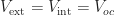
so that the terms including the series resistance (but not the parallel resistance!) become zero as well. Reordering the equation,

$j_\text{gen} = j_0 \left( \exp\left(\frac{qV_{oc}}{nkT} \right) -1 \right) - \frac{V_{oc}}{R_p}$ ,

we have an equation very similar to the diode equation (*). The pairs $j_\text{gen}(V_{oc})$ measured under a wide range of light intensities can, when shifted down by $j_{sc}(\text{1 sun})$ , correspond to the so called Suns-V_oc curve. It represents the $j(V_\text{int})$ curve, as the open circuit voltage is transport resistance free so that (only) there, $\Delta V=0$ . The Suns-V_oc curve is equivalent to the illuminated $j(V_\text{ext})$ curve, but lacks the influence of the series and transport resistance. The generation current $j_\text{gen} \approx eGL$ with the generation rate $G$ is sometimes (ok, often..) approximated by the short circuit current $j_{sc}$ .
An example of how a Suns-V_oc curve looks is shown in my earlier post on the diode ideality factor in the third figure (red = illuminated $j(V_\text{ext}$ ), green symbols = Suns-V_oc curve).

Of course there is a better way by measuring both the voltage dependent current and luminescence of a solar cell, as done by [Rau et al 2020] on Cu(In,Ga)Se₂ solar cells: from the luminescence, which depends on the quasi-Fermi level splitting, the internal voltage can be determined. For organic solar cells, as singlet and charge transfer exciton photoluminescence need to be separated – the internal voltage will be proportional to the latter – this is harder and has not been done yet, as far as I know.

How can the impact of the transport resistance on the fill factor, and thus performance, of organic solar cells be minimised? To reduce the transport resistance, the active layer conductivity needs to be increased. This can be done by, either, increasing the charge carrier mobility – for a molecular hopping system this means reducing static (low $\sigma$ ) and/or dynamic disorder (low $\lambda$ ). Or, increasing the carrier concentration – e.g. by doping, which is kind of hard in a bulk heterojunction, but starting with the material phase with the lower conductivity could be a viable approach.

Some hat tips here beyond the very nice cooperation of our study: Maria and Rod for feedback to an earlier version of the post, and Julien for being the first commenter on it:)

The diode ideality factor in organic solar cells: basics

Where does one start after so long an absence — meaning only the blog abstinence; I have been working and publishing since last time;-) One of the things which have been on my mind is the ideality factor, a figure of merit for the charge carrier recombination mechanism in a semiconductor diode. In short, a diode ideality factor of 1 is interpreted as direct recombination of electrons and holes across the bandgap. An ideality factor of 2 is interpreted as recombination through defects states, i.e. recombination centres. More on that in a later post, let’s start with the basics.

A couple of years ago, I wrote about some general properties of current-voltage characteristics of organic solar cells, but did not describe the ideality factor.¹ I think the ideality factor was mentioned only once, and then without details.

The Shockley diode equation describes the current–voltage characteristics of a diode,

$j=j_0 \left(\exp\left(\frac{eV}{n_{id}kT}\right)-1\right) - j_{gen}$ .

Here, $j$ current, $V$ the voltage, $e$ elementary charge, $kT$ thermal voltage, $j_0$ the dark saturation current, and $j_{gen}$ the photogenerated current. If the ideality factor $n_{id}$ was equal to one, one could call this the ideal Shockley equation. It derivation can be found in semiconductor text books, but it can also be derived based on thermodynamic arguments (see Peter Würfel’s excellent book on the physics of solar cells).

The current $j$ flowing out of the diode is defined to be negative. Essentially, the charge carriers which can flow out are the generated ones (e.g. $j_{gen}$ ), but reduced by the recombination current. That means,

$j=\underbrace{j_0 \left(\exp\left(\frac{eV}{n_{id}kT}\right)-1\right)}_{j_{rec}} - j_{gen}$ .

However, the term $j_{rec}$ contains also a negative contribution, $j_0$ times the $-1$ from the bracket. This is the thermal generation current $j_{gen,th} \equiv j_0$ , i.e. charge carriers excited across the bandgap just by thermal energy — and therefore very little. Still, the term is very important, as it is the prefactor of the whole $j(V)$ curve. Without light, i.e. with photocurrent $j_{gen}=0$ , we can clarify

$j=\underbrace{j_0 \exp\left(\frac{eV}{n_{id}kT}\right)}_{j_{rec,dark}} - \underbrace{j_0}_{j_{gen,th}}$ .

so that at negative voltages, $j=-j_0$ . Jdark (Please note that under realistic conditions, $j_0$ is not only pretty small and difficult to measure in principle, it is also hidden behind shunt currents in the device. ) At zero volt, $j=j_0-j_0=0$ . Thus, generation = recombination — or more specifically, thermal generation current = recombination current — which essentially implies that 0V correspond to the open circuit voltage in the dark.

How can one determine the ideality factor and the dark saturation current (at least in principle, see below for a better way on real devices)? It is common to neglect the thermal generation current (the term -1, multiplied by $j_0$ ), which is a good approximation for voltages some $kT/e$ larger than 0. Then, calculate the logarithm of the dark current ( $j_{gen}=0$ ),

$\ln(j) = \ln(j_0) +\frac{e}{n_{id}kT}V$ ,

so that the ideality factor can be determined from the inverse slope of the ln(current) at forward bias, and the dark saturation current from the current-axis offset. Let me already tell you that I do not recommend this approach, for reasons written below, and as explained in more detail in a recent paper of Kris Tvingstedt and myself [Tvingstedt/Deibel 2016].

Under illumination and at open circuit conditions, $j(V_{oc})=0$ , we can rewrite the Shockley equation as

$j_{gen}=j_0 \left(\exp\left(\frac{eV_{oc}}{n_{id}kT}\right)-1\right)$ ,

which has the same shape as the Shockley equation in the dark. This means that if you measure ( $j_{gen}, V_{oc}$ ) pairs for a (wide) range of different illumination intensities (thus varying $j_{gen}$ ), the points should overlap with the dark $j(V)$ curve! We’ll come back to this important point further below. Note that for solar cells with good fill factor, $j_{gen}$ can be approximated by the short circuit current $j_{sc}$ . Continue reading “The diode ideality factor in organic solar cells: basics”

Pseudosymmetry of the photocurrent physically relevant?

Two days ago, a paper considering the role of the “quasiflat band” case in bulk heterojunction solar cells by device simulations was published online [Petersen 2012]. It is critical of the pseudosymmetric photocurrent found and interpreted by [Ooi 2008] and later also ourselves [Limpinsel 2010]. In order to focus on the physical relevance of the (non)symmetry of the photocurrent, the paper by Petersen et al neglects a field dependent photogeneration. As some good points are raised, read the new paper if you are interested in the photocurrent.

[Update 2.4.2012] Another paper showing that band bending is not needed to explain the particular shape of the photocurrent: [Wehenkel 2012].

I will come back to field dependent photogeneration later, it is still intruiging: also here, the photocurrent should (and will be) complemented by pulsed measurements such as time delayed collection field, see e.g. [Kniepert 2011].

Add to Connotea

Charge transport in disordered organic matter: hopping transport

As I won a proposal today, I feel up to contributing once again some physics to this blog… I know, it has been a long long wait. So today it is time to consider some fundamentals of charge transport, as this is not only important for the extraction of charge carriers from the device (see earlier posts on mobility and efficiency, surface recombination velocity and photocurrent) but also the nongeminate recombination (see e.g. photocurrent part 2 and 3).

In disordered systems without long range order – such as an organic semiconductor which is processed into a thin film by sin coating – in which charge carriers are localised on different molecular sites, charge transport occurs by a hopping process. Due to the disorder, you can imagine that adjacent molecules are differently aligned and have varying distances across the device. Then, the charge carriers can only move by a combination of tunneling to cover the distance, and thermal activation to jump up in energy. In the 1950s, Rudolph A. Marcus proposed a hopping rate (jumps per second), which is suitable to describe the local charge transport. By the way, he received the 1992 Nobel prize in chemistry for his contributions to this theory of electron transfer reactions in chemical systems. Continue reading “Charge transport in disordered organic matter: hopping transport”

SPIE Pickings

Already 8 weeks past, recently some Videos (well, stills of the slides plus audio) of the Solar and LED Session of the SPIE Optics and Photonics 2011, San Diego went online.

Here are two or three which might interest you (well, they got my attention;-) but there is more to be found on the above mentioned web site – although I had to modify the settings of my ad blocker to be able to watch. No, there are no ads; still…

Before you scroll down, let me mention some other “findings” of potential interest:

How Google Went Solar by Dan Auld about Big G’s 1.65MW array, and how to get most out of it.
Then, a nice rant on the climate debate and how news media, trying to be biased, do become very biased… read Diamond planets, climate change and the scientific method by Matthew Bailes. You can see it as a kind of (inofficial) editorial for the last linked article, Who’s your expert? The difference between peer review and rhetoric by Ove Hoegh-Guldberg.
Another one on organic photovoltaics, Paper solar cells by 2015 (Disclaimer: I was involved in one of these projects. Um ;-).
Totally unrelated, PhDComics on Writing and Figures…
Even more unrelated, and not funny: Sitting and Standing at work, finally.
The most efficient flexible solar cells are not organic, but made from CIGS: Highly efficient Cu(In,Ga)Se2 solar cells grown on flexible polymer films (Nat Mater).
Alternatively, Silicon Ink can be used, as Bill Scanlon writes.
Stephen Wolfram on the Advance of the Data Civilization: A Timeline
Some lessons learned by Chris Dixon; while being about getting a job or your startup funded, it is somewhat applicable to carreers in science.
The Scientist on the Perfect Poster.
Nature News on the The reasons for retraction.

But now to these SPIE presentations [Update: WordPress does not accept the embedded vidos, so here just the links to the videos].

James Durrant, Imperial: Charge photogeneration and recombination in organic solar cells

Continue reading “SPIE Pickings”

Photocurrent again

I covered the photocurrent already before, for instance here. I pointed out that from the light intensity dependence of the short circuit current, it is impossible for many typical conditions to unambiguously determine the dominant loss mechanism or even the recombination order (1st (often called monomolecular, but not my favourite term;-) or 2nd order of decay).

If, however, you know (or guess) that the recombination order is two, you can use the above mentioned $j_{sc}$ vs. $P_L$ data to determine which fraction of charges is lost to bimolecular recombination, $\eta_{br}$ . This was shown recently by [Koster 2011]. For $j_{sc} \propto P_L^\alpha$ , they found $\eta_{br} = \alpha^{-1}-1$ . Although I was not able to follow the exact derivation ([Update 5.4.2011] it can be derived by solving a simple differential equation, $\alpha=(1-dR/dG)/(1-R/G)=(1-\eta_{br}')/(1-\eta_{br})$ ), it seems to work. Easy method, although make sure not to have too much space charge in your device – even at the contacts, induced by low (ohmic) injection barriers (we compared it to our device simulation, and then you get significant deviations)! In my opinion, the latter point is not stressed enough in the paper, despite the nice approach. Continue reading “Photocurrent again”

2011

A happy and successful new year to you! It is almost three years since I started this blog, this being the 69th post. A lot happened in this time, also for me: both personally (as some of the long term readers now;-) and professionally (despite still being in Würzburg;-). So, let me thank you, valued reader – and comments contributor, an active participation which I highly appreciate!

Many things I want to write about I have not had time to handle in the recent months. For now, let me start with just briefly revisiting what I have written. Hints of what I will add in the coming weeks and months are to come soon (soon meaning: worst case mid February, as one proposal is submitted by then, lecture is finished and project meeting / seminar talk marathon “finished”;-).

Find the overview below. Continue reading “2011”

Two notes

A few weeks ago, Heliatek managed to take the lead for organic solar cell efficiencies, achieving 8.3% confirmed power conversion efficiency on 1.1cm² active area with vacuum deposited small molecules. The device was a tandem. Thomas Körner, VP of Sales, marketing and Business Development at Heliatek, added

The first products should be coming onto the market at the start of 2012.

Good!

Second, you may remember my post on photocurrent in organic solar cells back in July. It was inspired by a comment I wrote on a paper by Street et al, who proposed monomolecular recombination to dominate the loss of free charges in organic bulk heterojunction solar cells. My comment and Bob Street’s reply to it are now online at Phys Rev B. I’ll not comment this interesting exchange any further (unless requested by you;-), so read and think for yourself!

Add to Connotea

	Transport resistance… on The transport resistance in or…
	Pitfalls when measur… on The transport resistance in or…
	deibel on The transport resistance in or…
	deibel on The transport resistance in or…
	Julien Gorenflot on The transport resistance in or…
	Julien Gorenflot on The transport resistance in or…
	deibel on The transport resistance in or…
	deibel on The transport resistance in or…
	Julien Gorenflot on The transport resistance in or…
	Julien Gorenflot on The transport resistance in or…