The last two times I wrote about transport resistance as a voltage-loss (or, depending on how you like to look at it, current-loss) mechanism in organic solar cells – in 2022 and 2025 – I mostly talked about fill factor: how a low active-layer conductivity bends the illuminated  curve around
  , and how the resulting gap between FF and pseudo-FF is often larger than the recombination loss itself, even in record-efficiency devices.
  This time I want to show you that a plot that is very common in today’s literature does not make much sense for today’s high-efficiency organic solar cells. I am talking about the plot of photocurrent – the difference between illuminated and dark current of a solar cell – vs what is called “effective voltage”, i.e.,
  vs.
vs.  . I mentioned this in a talk on transport resistance that I gave at the SAMSEC in Berlin in July 2025. I want to write this post to address potential misconceptions concerning this plot.
If you look at the current–voltage characteristics of state-of-the-art organic solar cells, as shown in the plot below, you can observe that dark and illuminated curves cross. The voltage at which they cross is often called  : it is the compensation voltage, and by definition, the photocurrent there is zero,
  . It is important to point out that in the ideal diode equation (briefly mentioned in this earlier post, equation “(*)”), this case never occurs: there, due to the superposition principle, the illuminated curve is just a shifted-down version of the dark current, by the generation current density
  . Thus, in the ideal case, dark and illuminated curve never meet!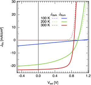
So, the question I hear you asking: why do the experimental dark and illuminated current densities cross?
For the field of organic photovoltaics, this question was first addressed by the Blom group, in Mihailetchi 2004. At this time, organic solar cells reached power conversion efficiencies of only 2 or 3%. So, Valentin Mihailetchi plotted the photocurrent density of a PPV:PCBM organic solar cell,  , against the effective voltage
  , where
  is the applied voltage. As result, one gets a photocurrent curve that rises steeply and then flattens into a plateau which corresponds to the solar cells’ maximum photocurrent. The authors interpreted this result as follows:
“The photocurrent in conjugated polymer-fullerene blends is dominated by the dissociation efficiency of bound electron-hole pairs at the donor–acceptor interface. A model based on Onsager’s theory of geminate charge recombination explains the observed field and temperature dependence of the photocurrent in PPV:PCBM blends. At room temperature only 60% of the generated bound electron-hole pairs are dissociated and contribute to the short-circuit current.”
The Mihailetchi model that was used to fit the photocurrent vs. effective voltage curve has two contributions. The first one goes back to Sokel and Hughes, is purely a drift-diffusion result for a device with no recombination and a voltage-independent generation rate  : with the internal field approximated by
  , the photocurrent is
![J_\mathrm{ph} = eGL\left[\dfrac{\exp(eV_\mathrm{eff}/kT)+1}{\exp(eV_\mathrm{eff}/kT)-1}-\dfrac{2kT}{eV_\mathrm{eff}}\right] \quad (1)](https://s0.wp.com/latex.php?latex=J_%5Cmathrm%7Bph%7D+%3D+eGL%5Cleft%5B%5Cdfrac%7B%5Cexp%28eV_%5Cmathrm%7Beff%7D%2FkT%29%2B1%7D%7B%5Cexp%28eV_%5Cmathrm%7Beff%7D%2FkT%29-1%7D-%5Cdfrac%7B2kT%7D%7BeV_%5Cmathrm%7Beff%7D%7D%5Cright%5D+%5Cquad+%281%29&bg=ffffff&fg=1a1a1a&s=0&c=20201002)
which is linear in close to (small internal field, diffusion-dominated) and saturates at  for larger (drift-dominated). Note that Eqn. (1) alone already produces the whole characteristic rise-then-plateau shape, with zero field-dependent physics anywhere in it. The second one is where Onsager–Braun comes in: since the experimental photocurrent kept rising beyond what Eq. (1) predicted, Mihailetchi et al. let the generation rate itself become field- and temperature-dependent,

with a dissociation probability for a bound polaron pair

so that  at high field, saturates at the true
  , and whatever fraction of
  you have reached at corresponding to short circuit is read off as “the dissociation probability” of the device. It is an elegant model, it fits the 2004 data very well, but today – two decades later – it is still the default lens through which people read any saturating – curve — even though, as Eq. (1) already shows, saturation on its own is not evidence of field-assisted dissociation at all.
So one thing is clear: you do not need field-dependent geminate pair dissociation to get this curve shape. The compensation voltage is nothing more exotic than the crossing point of two curves,  and
and  , and where that crossing sits is set largely by how the dark and illuminated currents change relative to one another at forward bias: This is a region where the transport resistance can play a major role.
In an ideal diode with no series or transport resistance, the dark and illuminated forward current keep climbing exponentially without bound, always separated by the generation current density. Formally,  . However, for a real solar cell, the active layer’s conductivity is low enough that transport resistance limits how much current can actually flow, the dark and illuminated current densities cross at the voltage . That pulls the crossing point down with decreasing conductivity (i.e.,
 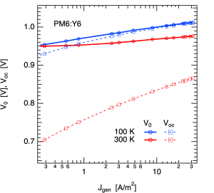 increasing transport resistance, for instance when lowering the temperature) until it sits just above — not because pair dissociation happens to saturate there.
We can observe exactly this behaviour in our own PM6:Y6 data: and come closer and closer for higher light intensity (or generation current), where the transport resistance becomes more pronounced. This trend can already be observed at 300 K, but the gap between them is closing rapidly at lower temperatures – here 100 K – where the active layer conductivity is much lower and the transport resistance higher.
We know from complementary measurements of the dissociation probability, shown for instance by Perdigón-Toro 2020 using the time delayed collection field (TDCF) technique, that the photogeneration in PM6:Y6 is virtually voltage independent. In terms of the Mihailetchi model, this would mean 
So, the presentation of vs. for modern organic solar cells carries no information on photogeneration. The reason for the crossing of dark and illuminated current is due to the transport resistance. To quantify the transport resistance, however, plotting the photocurrent vs. effective voltage is a much worse presentation and much less useful than investigating the slope of the illuminated curve around the open circuit voltage to directly determine the active layer conductivity. For details, I refer you to our original paper [Saladina 2025] and our perspective [Wang 2025]. My point is: stop using the vs. plot – it has lost its meaning for modern organic solar cells.
A toy model without dissociation
Another perspective to drive this point home. We built a very simple (toy:) model to discuss the expressiveness of the Mihailetchi plot: a single-diode device (dark current ![J_\mathrm{dark}=J_{00}\exp(-E_\mathrm{g}/nkT)\,[\exp(eV_\mathrm{i}/nkT)-1]](https://s0.wp.com/latex.php?latex=J_%5Cmathrm%7Bdark%7D%3DJ_%7B00%7D%5Cexp%28-E_%5Cmathrm%7Bg%7D%2FnkT%29%5C%2C%5B%5Cexp%28eV_%5Cmathrm%7Bi%7D%2FnkT%29-1%5D&bg=ffffff&fg=1a1a1a&s=0&c=20201002) , plus a fixed generation current subtracted under illumination, exactly as in the standard superposition approximation, but coupled to a transport bottleneck: the active layer is given a conductivity
, plus a fixed generation current subtracted under illumination, exactly as in the standard superposition approximation, but coupled to a transport bottleneck: the active layer is given a conductivity  that is translated into a voltage dependent series resistance – the transport resistance! Every internal voltage
  is mapped to an external, applied voltage via
  — a voltage drop across the active layer that grows with the local current and shrinks with the local conductivity. This exactly corresponds to the transport-resistance picture.
 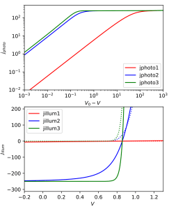 Crucially, itself never depends on voltage or on
  : there is no Onsager–Braun physics anywhere in this model, no bound pairs, nothing to dissociate. If the Onsager–Braun picture were the only thing that can produce a saturating – curve, sweeping the conductivity prefactor in this toy device should do nothing to its – shape.
It does the opposite. Changing the conductivity prefactor over five orders of magnitude (at fixed illumination and temperature) reproduces the textbook saturating “Mihailetchi curve” for every (of the three shown) conductivity values, just shifted depending on the magnitude of conductivity.
The numbers make the point sharper than the shapes alone. Going from the best-transport end of the variation to the worst, the fill factor drops very strongly, and the compensation voltage is pulled down from hundreds ov milliVolts above to “barely above it” — while itself does not change (as the illumination remains the same). That last point matters: transport resistance is overwhelmingly a fill-factor and current problem, not a voltage problem.
Take home message
I find the vs. plot in almost every high efficiency organic solar cell paper that I open. Usually, the accompanying explanation reads something like:
“The photon-to-electron conversion efficiency of our organic solar cells is governed by exciton dissociation and charge collection. Accordingly, the charge-dissociation probability,  , and charge-collection probability,
  , of all devices were determined from plots of photocurrent density as a function of effective voltage. Among the investigated devices, the best one achieved the highest values, with
  and
and  .”
.”
This is incorrect and cannot be determined with the model at all. If you want to make a statement on dissociation efficiency, please measure it with TDCF or similar. If you really want to make a statement on collection losses: these are dominated by transport resistance losses, so look into which figures of merit are useful to quantify the contributions to the fill factor – losses due to (small part) recombination and (large part) a low active layer conductivity. If you want the full toolbox for recognising and quantifying transport resistance losses, Maria’s review has it all: how to predict pseudo-FF from the recombination ideality factor, how to get the active-layer conductivity out of the transport resistance, why  is voltage-dependent, how energetic disorder feeds into it, and how to minimise the loss in the first place [Saladina 2025].
As always, I am happy to hear your thoughts.